Buying a house ?

A good old regression problem is the house prices prediction. I chose to tackle this one using Kaggle’s data set, available here.
The data set describes residential homes in Ames (Iowa) using 79 explanatory features. The goal is to predict the price for each home.

What is provided:
– Training data set: includes sales price for each home.
– Test data set: doesn’t include sales price. To be predicted.
– Description: of all features in data set. There are 79 features, and it can be heavy at first, but it is essential to go through each one to understand it at first, and see how it can be used later.

There is a little bit more than 1400 rows in each data set. I would have preferred a larger data set, as there are a lot of features, to avoid over fitting.
Unless each feature explains just a little bit of the final price, there must be a way to do a good feature selection, I will explore that point later.
I should tell that I have started with a very basic modeling solution, without feature engineering to get a sense of the problem. Then, I introduced enhancements described below in each section.

Libraries

import pandas as pd
from sklearn.linear_model import LinearRegression, Ridge, Lasso, ElasticNet
from matplotlib import pyplot as plt
import seaborn as sb
from statsmodels.graphics.gofplots import qqplot
from scipy.stats import skew, boxcox
from scipy.special import boxcox1p
from sklearn import feature_selection, model_selection, metrics

Data preparation :

There are 2 types of features : numeric and categorical.
I regrouped both training and testing data in order to apply transformations to both.

train = pd.read_csv(r"Path_to_file\train.csv")
size_train = len(train)
test = pd.read_csv(r"Path_to_file\test.csv")
size_test = len(test)
data = pd.concat([train[train.columns.difference(["SalePrice"])], test], ignore_index=True, sort=False)

Keeping the original sizes of train and test set is helpful to split data again later.

Features with incorrect type

Some features can’t be considered as numerical, yet they are in the data set as numeric data. Keeping the numeric type introduces order while there is none in reality. I changed the type to string.
– MSSubClass: the type of dwelling involved in the sale.
– MoSold: sale’s month, from 1 to 12.
– YrSold: sale’s year (very few values compared to other year date features).

         Count
YrSold     
2006    619
2007    692
2008    622
2009    647
2010    339

# should not be stored as number, introduces ordinality when there is none. 
data["MSSubClass"] = data["MSSubClass"].apply(str)
data["MoSold"] = data["MoSold"].apply(str)
data["YrSold"] = data["YrSold"].apply(str)

Missing data

Most of features have indications to apply when data is missing in the description document :
– If empty means None (if categorical) or 0 (if numerical). That is the case for the house elements (garage, basement, pool, bathroom …) such as : Alley, Fence, PoolQC, FireplaceQu, BsmtFinType1, GarageQual, MiscVal, MiscFeature …
– If empty means Typical. That is the case for Functional.
– If empty just means that data is missing. I chose to replace the empty value with most frequent value or median.

# to check for missing data
missing_col = (data.isna().sum()) * 100 / (size_train+size_test)
print(missing_col[missing_col !=0].sort_values(ascending=False))

The result :

                % of missing data
Feature
PoolQC          99.657417
MiscFeature     96.402878
Alley           93.216855
Fence           80.438506
FireplaceQu     48.646797
LotFrontage     16.649538
GarageQual       5.447071
GarageCond       5.447071
GarageFinish     5.447071
GarageYrBlt      5.447071
GarageType       5.378554
BsmtExposure     2.809181
BsmtCond         2.809181
BsmtQual         2.774923
BsmtFinType2     2.740665
BsmtFinType1     2.706406
MasVnrType       0.822199
MasVnrArea       0.787941
MSZoning         0.137033
BsmtFullBath     0.068517
BsmtHalfBath     0.068517
Utilities        0.068517
Functional       0.068517
Electrical       0.034258
BsmtUnfSF        0.034258
Exterior1st      0.034258
Exterior2nd      0.034258
TotalBsmtSF      0.034258
GarageArea       0.034258
GarageCars       0.034258
BsmtFinSF2       0.034258
BsmtFinSF1       0.034258
KitchenQual      0.034258
SaleType         0.034258

It is possible to do mass update depending on the variable data type. Personally, since I checked variable by variable at first, I managed each one by itself.
To be consistent, I used only train data to calculate median and most frequent value, not both train and test sets.

def fill_missing_values(data, train):
    # replace LotFrontage with median value
    data["LotFrontage"] = data["LotFrontage"].fillna(train["LotFrontage"].median())
    # replace MasVnrType with most frequent value 
    # replace MasVnrArea with median of most frequent value for MasVnrType (None)
    data["MasVnrType"] = data["MasVnrType"].fillna(train["MasVnrType"].value_counts().index[0])
    data["MasVnrArea"] = data["MasVnrArea"].fillna(train[train.MasVnrType=="None"].MasVnrArea.median())
    # replace with most common value
    fill_with_most_frequent = {"Electrical","KitchenQual","Exterior1st","Exterior2nd","SaleType","MSZoning","Utilities"}
    for feature in fill_with_most_frequent:
        data[feature] = data[feature].fillna(train[feature].value_counts().index[0]) 
    data["Functional"] = data["Functional"].fillna('Typ') # according to data description
    data["Utilities"] = data["Utilities"].fillna(train["Utilities"].value_counts().index[0])
    # fill other missing values with correspondance : NA = 0
    fill_with_none = {"Alley","Fence","PoolQC","FireplaceQu","BsmtFinType1","BsmtFinType2","BsmtQual","BsmtCond","BsmtExposure","GarageCond","GarageFinish","GarageType","GarageQual","MiscFeature"}
    fill_with_zero = {"BsmtFinSF1","BsmtFinSF2","BsmtFullBath","BsmtHalfBath","BsmtUnfSF","GarageArea","GarageCars","TotalBsmtSF","GarageYrBlt","MiscVal"}
    for feature in fill_with_none:
        data[feature] = data[feature].fillna("None")
    for feature in fill_with_zero:
        data[feature] = data[feature].fillna(0)
    # drop unused features : Id
    data.drop(["Id"], axis=1, inplace=True)
    return data

Feature engineering

By working the data better, the model may perform better as it easier to recognize patterns. To check if this is helpful in my case, I added to initial features new ones :
– BathNum as the total of bathrooms.
– Porch as the total porch area.
– TotalSF as the total square feet area of the house.
– HasGarage as a binary variable indicating if the house has a garage.
– HasFirePlace as a binary variable indicating if the house has a fireplace.
As a result, I dropped the initial features in the operation except TotalBsmtSF, 1stFlrSF and 2ndFlrSF. I confirmed this intuition when I saw how skewed the variables were (next section) and also by testing the model with and without them. Indeed, I saw an increase in my predictions performance when they were removed.

At first, I also added:
– HasPool : as a binary variable indicating if the house has a pool.
– HasBsmt : as a binary variable indicating if the house has a basement.
But I didn’t keep them at the end as I will explain later.

def feature_eng(data):
 data["BathNum"] =data['FullBath'] + (0.5 * data['HalfBath']) + data['BsmtFullBath'] + (0.5 * data['BsmtHalfBath'])
 data["Porch"] = data['OpenPorchSF'] + data['3SsnPorch'] + data['EnclosedPorch'] + data['ScreenPorch'] + data['WoodDeckSF']
 data["TotalSF"] = data['TotalBsmtSF'] + data['1stFlrSF'] + data['2ndFlrSF']
 data["HasGarage"] = data["GarageArea"].apply(lambda x : 1 if x > 0 else 0)
 data["HasFirePlace"] = data["Fireplaces"].apply(lambda x: 1 if x > 0 else 0)
 data.drop(["FullBath","HalfBath","BsmtFullBath","BsmtHalfBath","OpenPorchSF","3SsnPorch","EnclosedPorch","WoodDeckSF"], axis =1, inplace=True)
 return data

Skewness for numeric features

The regression techniques I’ll use in modeling section perform better with pseudo-normal or normal distributions. Either visually or numerically, it appears that some features are highly skewed.
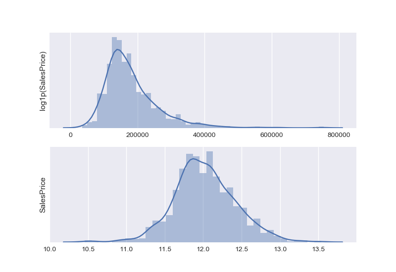
First, let’s check the distribution of SalesPrice in the data set. It seems skewed and far from a centered normal distribution. Applying the log transformation helps though.
As for features, I performed cox box transformation and dropped the ones that still represented skewness after the transformation.

For Y

Y = np.log1p(train["SalePrice"])

For features

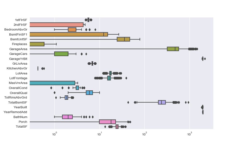
It is a bit more complicated for features, as some of them are not only far from a normal distribution (QQ-plot below), but also highly skewed (box plot below).

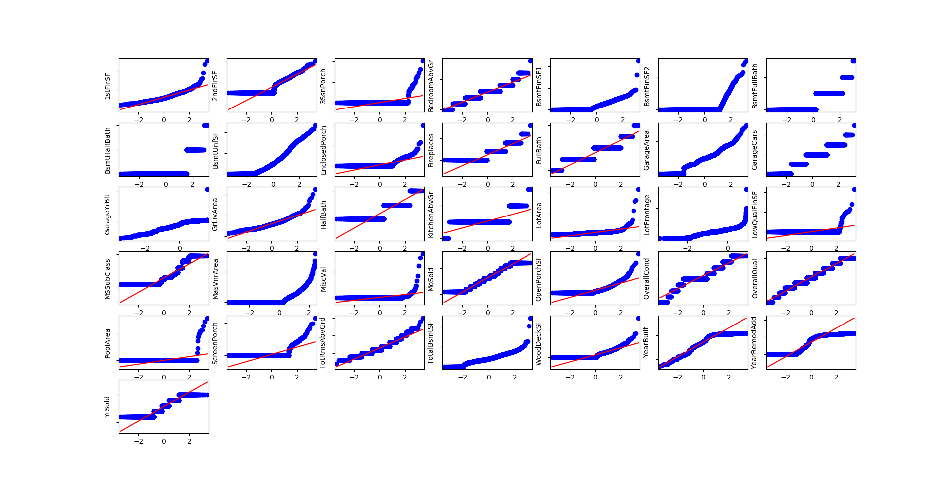
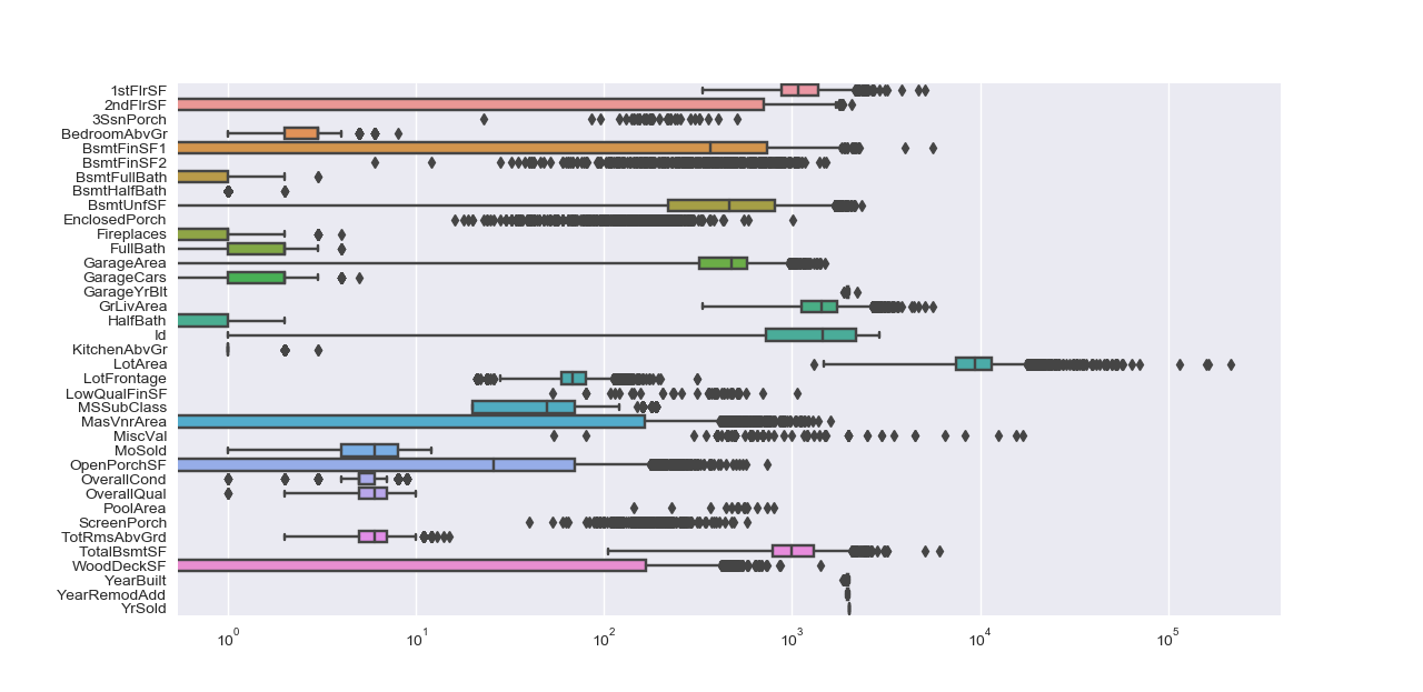
I chose to apply box-cox transformation for highly skewed distributions and ended up dropping features that were still strong skewed after this transformation.

def apply_boxcox(data):
     """ Applies cox box transformation to features """
     num = ['int16', 'int32', 'int64', 'float16', 'float32', 'float64']
     cols = data.select_dtypes(include=num).columns.values  
     for var in cols:
         skewness = skew(data.loc[:,var])
         if skewness > 0.5:
             data.loc[:,var],_ = boxcox(data.loc[:,var]+1) # +1 to manage 0 values
             # drop columns that are skewed after cox box transformation.
             if skew(data.loc[:,var]) > 0.5:
                 data.drop([var], inplace=True, axis = 1)
     return data

Removing single values columns

I also decided to remove columns that have a dominant value, meaning that the most frequent value represents more than 95% of the feature. That is the reason why I didn’t keep HasBsmt and HasPool.

def remove_singlevalue(data):
    for col in data.columns:
        if data[col].value_counts().iloc[0] >= (95 * len(data[col]) / 100):
            data.drop(col, axis=1, inplace = True)
    return data

Condition2
Heating
KitchenAbvGr
LandSlope
MiscFeature
PoolQC
RoofMatl
Street
Utilities

Transform categorical features

It is possible to perform one hot encoding for some features. It could be meaningful for some, such as KitchenQual, GarageCond, BsmtCond … but I finally decided to use the dummy features instead.
In fact, I tested both and they both gave me the same results.

def transform_categorical(data):
 return pd.get_dummies(data=data)  

Scaling

Since features are on different scales, this step is important. I scale both training and testing sets using the mean and standard deviation of the training set.

def scale(train, test):
 means = train.mean()
 stdevs = train.std()
 train = (train.subtract(means,axis=1)).divide(stdevs,axis=1)
 test = (test.subtract(means,axis=1)).divide(stdevs,axis=1)
 return train, test

Removing outliers

This was tricky as there are multiple ways to tackle this. First, the creator of the data set gave a recommendation: to remove from the training set, houses with GrLivArea > 4000, defining them as outliers. Indeed, we can see it in the scatter plot between SalePrice and GrLivArea.

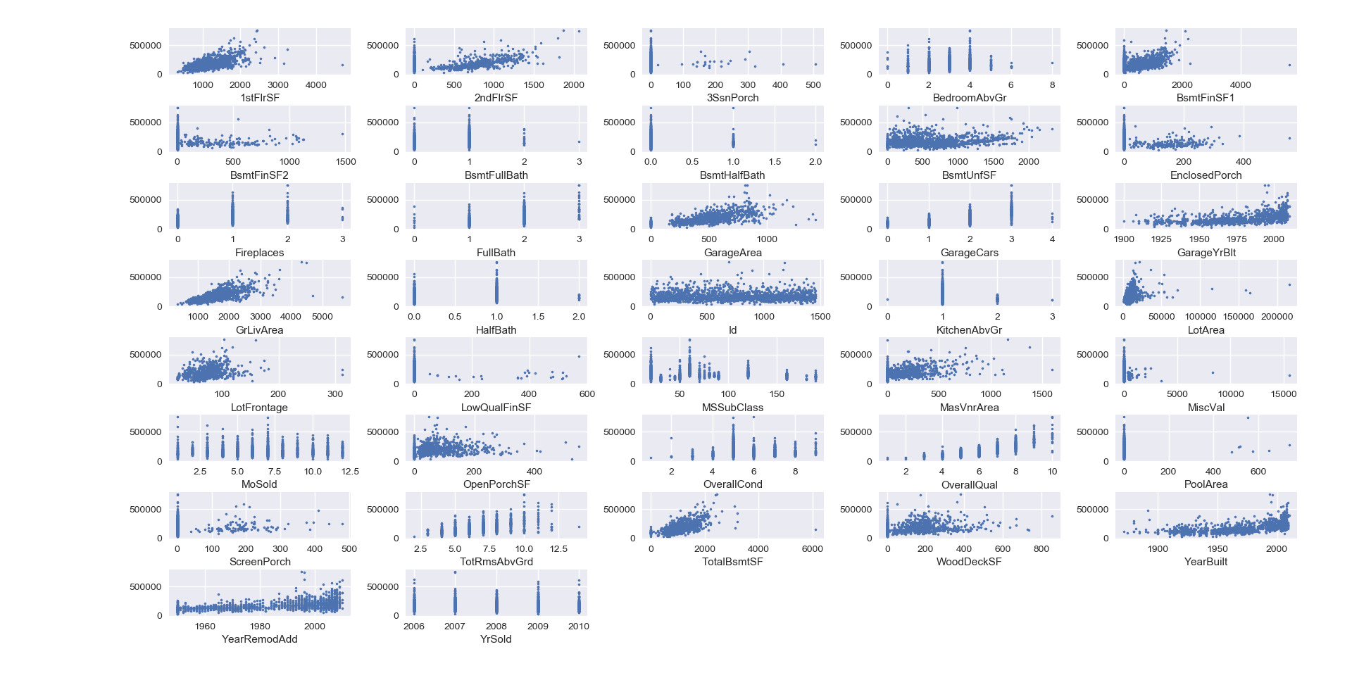
More generally, outliers are easily spotted using the other features as well with scatter plot. But then, they have to be removed manually from the data set.

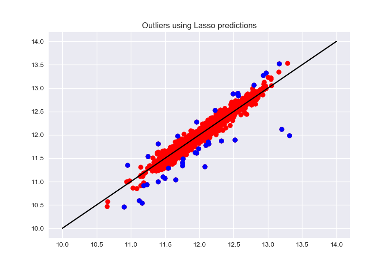
I also tried another method which consists of using a simple regression model to predict the house price on the training set, then, remove rows for which the prediction is far away from the initial sales prices.
Meaning, calculate the residuals between the actual and predicted price, scale them and spot the ones that are larger/smaller than 3 times the standard deviation of residuals.

def remove_outliers(X,y,sigma):
     range_alpha = np.logspace(-3, 3, 50)
     param_grid = {'alpha': range_alpha}
     model_lasso = model_selection.GridSearchCV(Lasso(), param_grid, cv=5)
     model_lasso.fit(X, y)
     pred = model_lasso.predict(X)
     residuals = pred - y
     std_dev_res = residuals.std()
     mean_res = residuals.mean()
     Z = (residuals - mean_res)/std_dev_res
     X.drop(Z[abs(Z) > sigma * abs(Z).std()].index, inplace=True)
     y.drop(Z[abs(Z) > sigma * abs(Z).std()].index, inplace=True)
     return X, y

Feature selection

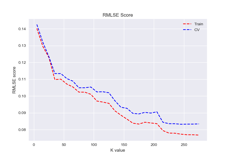
I tried also feature selection to see if there is way to reduce the number of features. The graph shows that cross validation error becomes more or less constant starting from 217 features.
I also double checked that with test error and it is consistent.
However, this didn’t do much to the model performance that we will see in the next section.

# Feature selection
def selectK(x,y,Kgrid, param_grid):
    errors = pd.DataFrame(columns=['k','train_rmsle','test_rmsle'])
    for k in Kgrid:
        Kbest = feature_selection.SelectKBest(feature_selection.f_regression, k=k)
        X_new = Kbest.fit_transform(x, y)
        X_train, X_test, y_train, y_test = model_selection.train_test_split(X_new, y, test_size=0.3,random_state=42)
        model = model_selection.GridSearchCV(Lasso(), param_grid, cv=5)
        model.fit(X_train, y_train)
        print(k)
        print(model.best_params_)
        # cross validation
        y_cv = model.predict(X_test)
        y_train_pred = model.predict(X_train)
        cv_rmsle = np.sqrt(metrics.mean_squared_log_error(np.expm1(y_test), np.expm1( y_cv)))
        train_rmsle = np.sqrt(metrics.mean_squared_log_error(np.expm1(y_train), np.expm1(y_train_pred)))
        errors = errors.append([pd.Series([k, train_rmsle, cv_rmsle], index = errors.columns)])
    return errors

Modeling

First, I go back to the initial configuration: meaning a training set and a test set. Then I split my training data into 2 sets : usually 70% for training purposes and 30% for cross validation.
It is important to assess the model using data that it has never “seen”. So, for each model, there will be a training error and a cross validation error.
This also helps me check if there is over fitting (very small training error and very high cross validation error).
To estimate the model’s performance, I use (as Kaggle score method) the root mean square log error RMSLE.

X_scaled, X_pred_scaled = process.scale(X, X_pred)
X_train, X_test, y_train, y_test = model_selection.train_test_split(X_scaled,Y,test_size=0.3, random_state=41)

Ridge

A Linear least squares with l2 regularization, more information available here.

range_alpha = np.logspace(-3, 3, 50)
param_grid= {'alpha': range_alpha }
model = model_selection.GridSearchCV(Ridge(), param_grid, cv=5)
model.fit(X_train,y_train)
y_cv = model.predict(X_test)
y_train_pred = model.predict(X_train)
cv_rmsle = np.sqrt(metrics.mean_squared_log_error(np.expm1(y_test),np.expm1(y_cv)))
train_rmsle = np.sqrt(metrics.mean_squared_log_error(np.expm1(y_train),np.expm1(y_train_pred)))

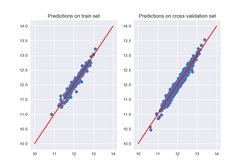
Training error, cross validation error and optimal value for alpha (parameter tuning):

Ridge train_rmsle on train set: 0.07033602804422778
Ridge cv_rmsle on cv set: 0.08726205991464978
{'alpha': 33.9322177189533}

Lasso

A Linear Model trained with L1 prior as regularizer , more information available here.

range_alpha = np.logspace(-3, 3, 50)
param_grid= {'alpha': range_alpha }
model_lasso = model_selection.GridSearchCV(Lasso(), param_grid, cv=5)
model_lasso.fit(X_train,y_train)
y_cv_lasso = model_lasso.predict(X_test)
y_train_pred_lasso = model_lasso.predict(X_train)
cv_rmsle_lasso = np.sqrt(metrics.mean_squared_log_error(np.expm1(y_test),np.expm1(y_cv_lasso)))
train_rmsle_lasso = np.sqrt(metrics.mean_squared_log_error(np.expm1(y_train),np.expm1(y_train_pred_lasso)))

Training error, cross validation error and optimal value for alpha (parameter tuning) :

Lasso train_rmsle on train set: 0.0750237156813598
Lasso cv_rmsle on cv set: 0.08509427639976841
{'alpha': 0.002329951810515372}

Elastic Net

A Linear regression with combined L1 and L2 priors as regularizer, more information available here.

range_alpha = np.logspace(-3, 3, 50)
range_l1_ratio = np.logspace(-1, -0.1, 50)
param_grid_en= {'alpha': range_alpha, 'l1_ratio':range_l1_ratio }
model_en = model_selection.GridSearchCV(ElasticNet(), param_grid_en, cv=5)
model_en.fit(X_train, y_train)
y_cv_en = model_en.predict(X_test)
y_train_pred_en = model_en.predict(X_train)
cv_rmsle_en = np.sqrt(metrics.mean_squared_log_error(np.expm1(y_test),np.expm1(y_cv_en)))
train_rmsle_en = np.sqrt(metrics.mean_squared_log_error(np.expm1(y_train),np.expm1(y_train_pred_en)))

Training error, cross validation error and optimal value for alpha and l1_ratio (parameter tuning):

Elastic Net  train_rmsle on train set: 0.07533996988643514
Elastic Net  CV_rmsle on cv set: 0.0853127780792455
{'alpha': 0.0030888435964774815, 'l1_ratio': 0.7943282347242815}

Solo, the best model after tuning is Lasso.
But then, out of curiosity, I wanted to check if stacking would help. What if each model is a poor learner and combining them would make a strong learner ?
Since Lasso and Elastic Net performed the best on cross validation, I chose to combine the predictions of the 2 models into a new training set and predict the final sales price from it using Ridge.

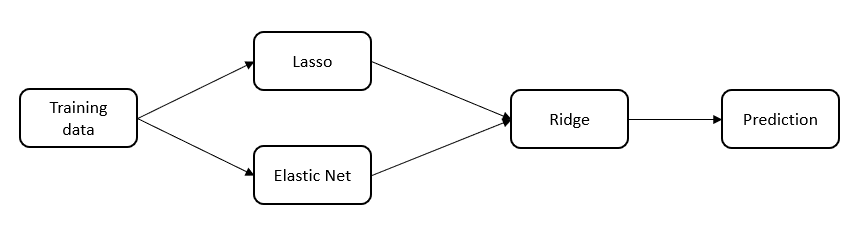
model = model_selection.GridSearchCV(Ridge(), param_grid, cv=5)
X_stack = pd.concat([pd.DataFrame(y_train_pred_lasso),pd.DataFrame(y_train_pred_en)]
                     ,ignore_index=True, sort=False, axis =1)
X_cv = pd.concat([pd.DataFrame(model_lasso.predict(X_test)), pd.DataFrame(model_en.predict(X_test))],ignore_index=True,
                  sort=False, axis=1)
model.fit(X_stack,y_train)
y_cv = model.predict(X_cv)
y_train_pred = model.predict(X_stack)
cv_rmsle = np.sqrt(metrics.mean_squared_log_error(np.expm1(y_test),np.expm1(y_cv)))
train_rmsle = np.sqrt(metrics.mean_squared_log_error(np.expm1(y_train),np.expm1(y_train_pred)))

Ridge stacking  train_rmsle on train set: 0.0732295078690761
Ridge stacking cv_rmsle on cv set: 0.08439024246853641

The cross validation error is better but, not by far from the single Lasso model.

Prediction

Now, is is time to make predictions on the test set :

X_pred_stack = pd.concat([pd.DataFrame(model_lasso.predict(X_pred_scaled)), pd.DataFrame(model_en.predict(X_pred_scaled))]
                          ,ignore_index=True, sort=False,axis =1)
y_pred = np.expm1(model.predict(X_pred_stack))
y_pred = pd.DataFrame(y_pred, columns=["SalePrice"])
y_pred.insert(0, "Id", test["Id"])
y_pred.to_csv("y_pred.csv", index=False)

The predictions on the test set scored 0.11918 on Kaggle Leaderboard.

Extra comments

It is possible to try adding degree to features (polynomial for instance), but I didn’t pursue this possibility as the data set isn’t large enough and that could lead to a high bias model, which causes over fitting.

Thanks for reading this post and see you soon !