I wanted to start tackling NLP (NLP for natural language processing) problems for a while now. And what could be better than a sentiment analysis problem, a simple binary classification problem using tweets ? The goal here is to predict whether a tweet is about a real disaster or not. This is particularly useful for media platforms who could investigate further based on a simple alarm.

What we have is a data set for training of 7613 rows and 5 columns, 2 of which we will use:
– text : the tweet itself
– target: 1 for a disaster tweet and 0 otherwise.
The remaining columns (unused here) are id, keyword and location.
There is also a test data set without the the variable target.
All details can be found here.
Data preparation
Let’s start by importing the libraries needed and loading the training data :
import pandas as pd
import matplotlib
matplotlib.use("TkAgg")
from matplotlib import pyplot as plt
import seaborn as sns
import numpy as np
from sklearn import feature_extraction
train = pd.read_csv("data/train.csv")
test = pd.read_csv("test.csv")
Let’s check what the data looks like, a random row from train :
id                                                   16
keyword                                             NaN
location                                            NaN
text        Three people died from the heat wave so far
target                                                1
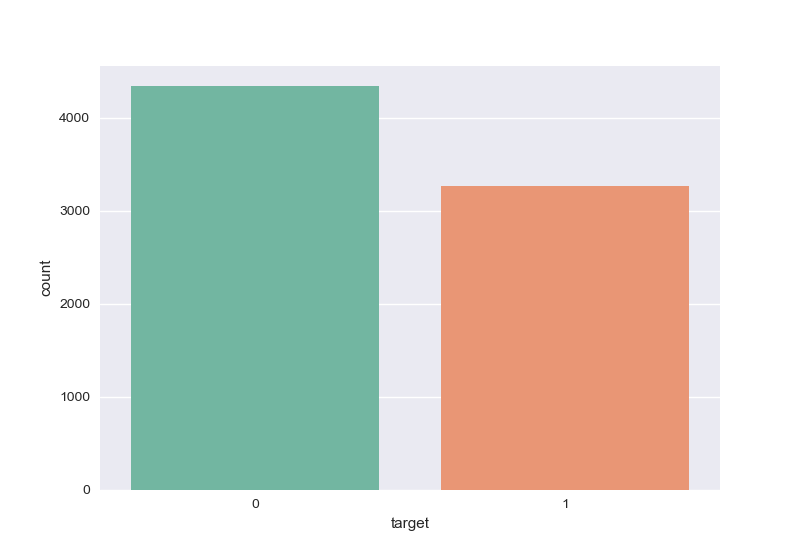
How many tweets are about a disaster in the training data set ? It looks like this is a balanced data set :
plt.style.use("seaborn")
sns.countplot(x='target', data=train, palette="Set2")
plt.show()
As we are working with tweets, there could be usernames as well as URL links in the variable text. Let’s get rid of those to explore data.
# remove http/s www links for data exploration
train["text"] = train["text"].replace(r'http\S+', '<>', regex=True).replace(r'www\S+', '<url>', regex=True)
# remove user names with void for data exploration
train["text"] = train["text"].replace(r'@\S+', '<>', regex=True)
Data exploration
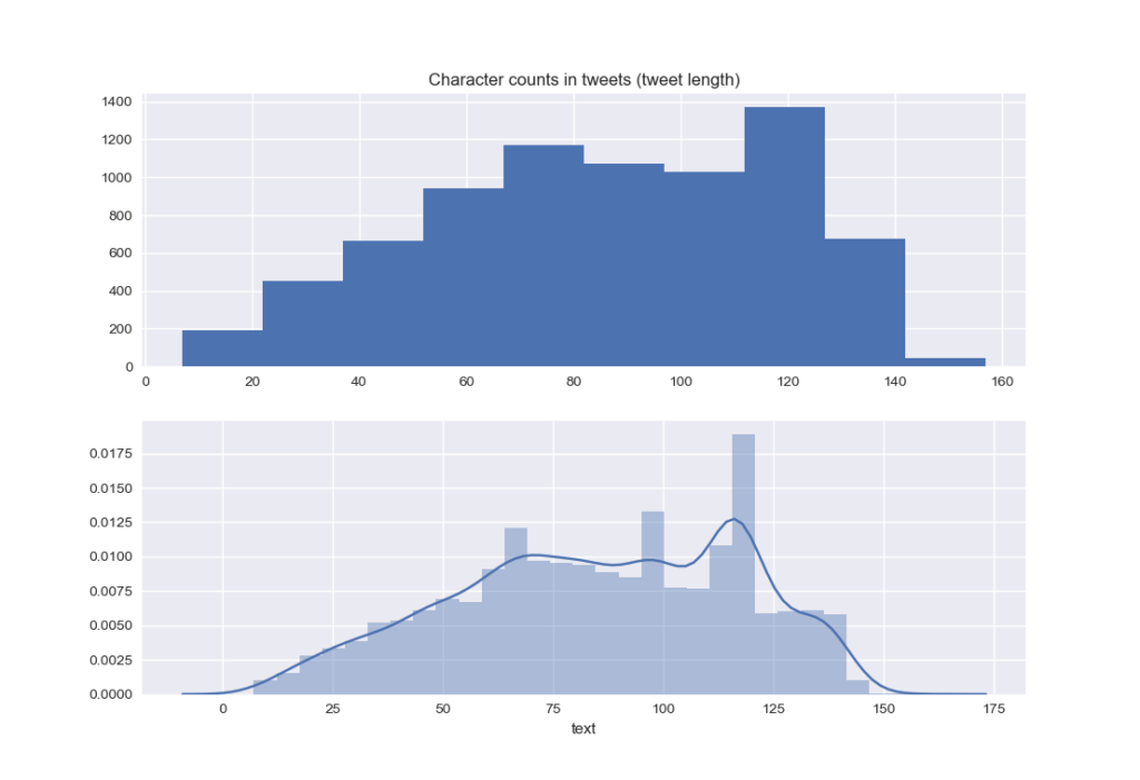
The distribution of the length for each tweet (number of characters) : a lot of the tweets go from 20 to 125 characters.
plt.clf()
char_count = train['text'].str.len()
plt.subplot(2, 1, 1)
plt.title('Character counts in tweets (tweet length)')
plt.hist(char_count)
plt.subplot(2, 1, 2)
sns.distplot(char_count)
plt.show()
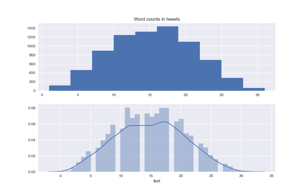
The number of words per tweet has the following distribution :
plt.clf()
word_count = train['text'].str.split().apply(lambda x: len(x))
plt.subplot(2, 1, 1)
plt.title('Word counts in tweets')
plt.hist(word_count)
plt.subplot(2, 1, 2)
sns.distplot(word_count)
plt.show()
As for the average of word length in the tweets :
plt.clf()
word_length = train['text'].str.split().apply(lambda x: [len(i) for i in x]).apply(lambda x: np.mean(x))
plt.subplot(2, 1, 1)
plt.title('Word length average by tweet')
plt.hist(word_length)
plt.subplot(2, 1, 2)
sns.distplot(word_length)
plt.show()
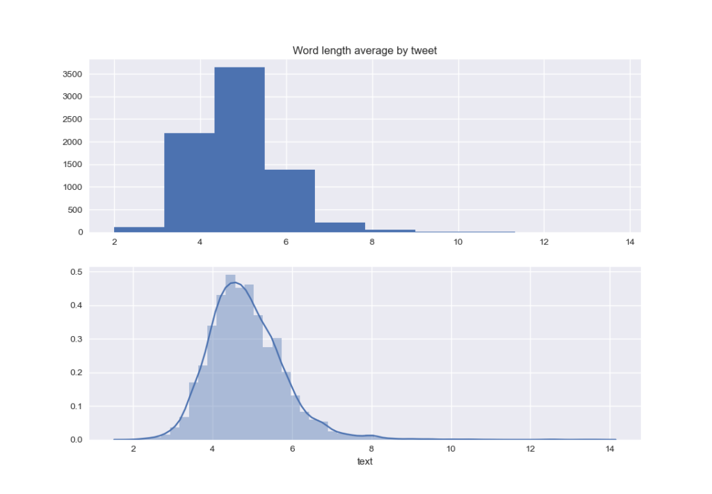
It seems that most of words are not very long. Still, there are very few which explains the skewed distribution.
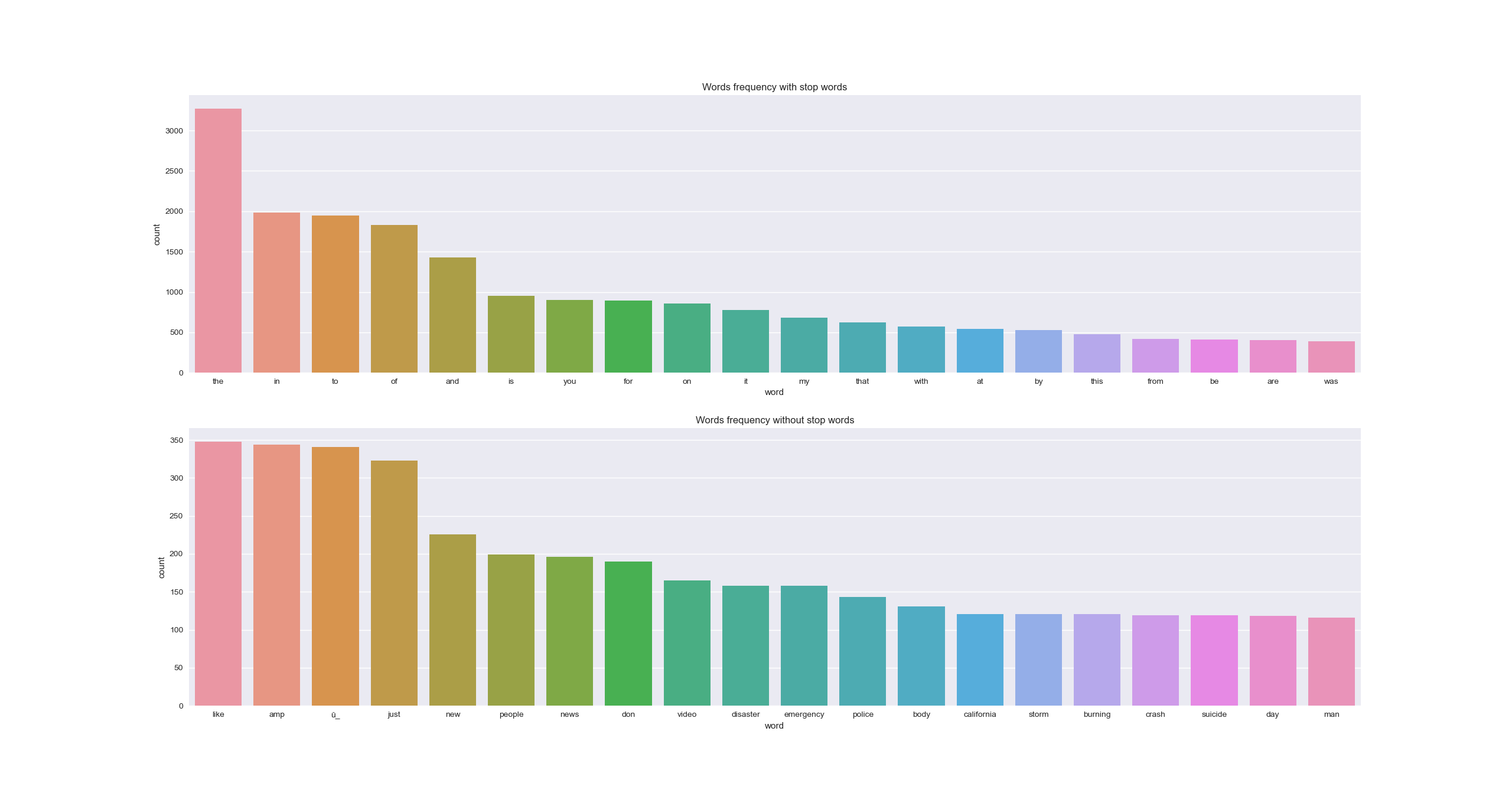
A good point could be to check what the most frequent words are. For that, we plot 1-gram and 2-gram diagrams. As the presence of stop words can be misleading, we will check the n-grams both before and after removing the stop words from tweets. As a remainder, the stop words are the most common words in a language, which most search engines are programmed to ignore.
def get_freq_words(data, n, without_stop_words, gram):
    if without_stop_words:
        vec = feature_extraction.text.CountVectorizer(stop_words='english', ngram_range=gram).fit(data)
    else:
        vec = feature_extraction.text.CountVectorizer(ngram_range=gram).fit(data)
    words = vec.transform(data)
    sum_words = words.sum(axis=0)
    words_freq = [(word, sum_words[0, idx]) for word, idx in vec.vocabulary_.items()]
    words_freq = sorted(words_freq, key=lambda x: x[1], reverse=True)
    words_freq_df = pd.DataFrame(words_freq, columns=['word', 'count'])
    words_freq_df.drop(words_freq_df[(words_freq_df['word'] == 'user') | (words_freq_df['word'] == 'url')].index,
                       inplace=True)
    return words_freq_df[:n]


n = 20
with_stop_words = get_freq_words(train['text'], n, False, (1, 1))
without_stop_words = get_freq_words(train['text'], n, True, (1, 1))
plt.clf()
plt.subplot(2, 1, 1)
sns.barplot(with_stop_words['word'], with_stop_words['count'])
plt.title('Words frequency with stop words')
plt.subplot(2, 1, 2)
sns.barplot(without_stop_words['word'], without_stop_words['count'])
plt.title('Words frequency without stop words')
plt.show()
n = 20
bi_with_stop_words = get_freq_words(train['text'], n, False, (2, 2))
bi_without_stop_words = get_freq_words(train['text'], n, True, (2, 2))
plt.clf()
plt.subplot(2, 1, 1)
sns.barplot(bi_with_stop_words['word'], bi_with_stop_words['count'])
plt.xticks(rotation=45)
plt.title('Bi-grams frequency with stop words')
plt.subplot(2, 1, 2)
sns.barplot(bi_without_stop_words['word'], bi_without_stop_words['count'])
plt.xticks(rotation=45)
plt.title('Bi-grams frequency without stop words')
plt.show()
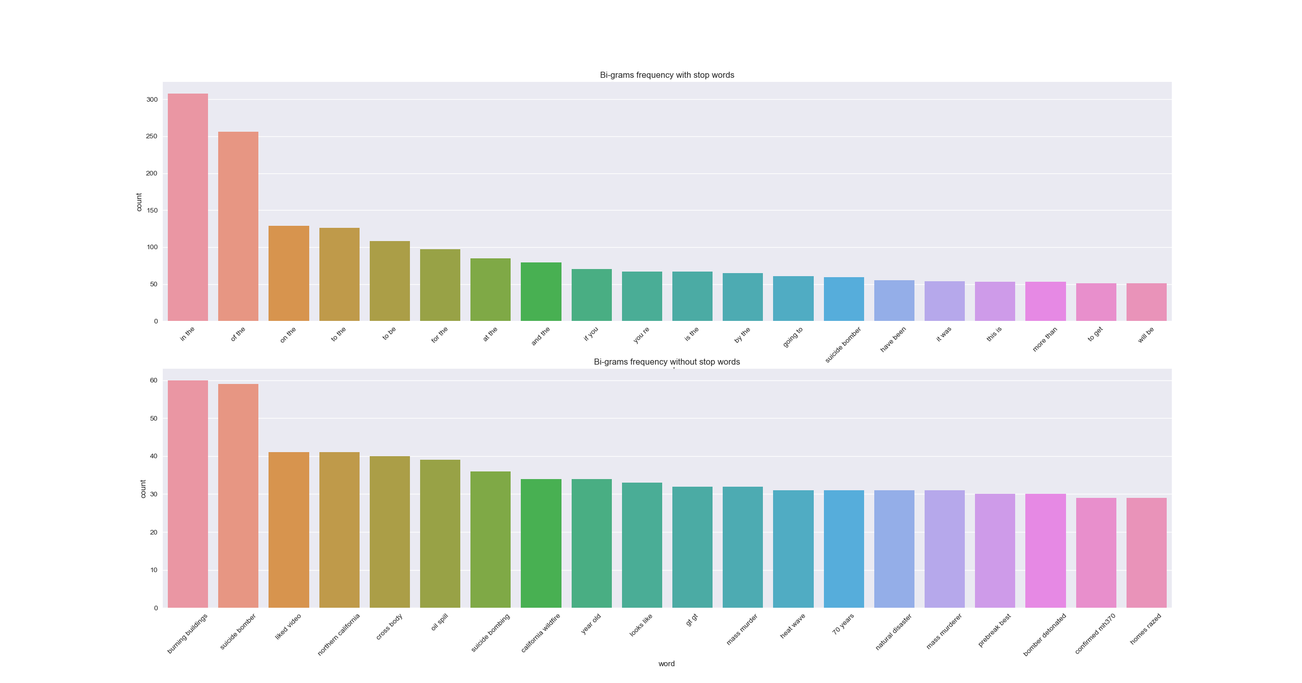
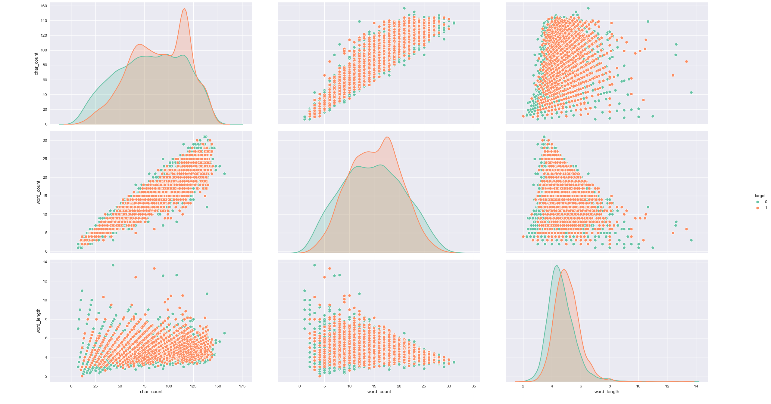
Both the mono and bi-grams pick up some of the disaster words. It is more obvious in the bi-grams. But are there any obvious clusters based on the number of words, characters or average length ? Not really.
df = pd.DataFrame(
    {'char_count': char_count, 'word_count': word_count, 'word_length': word_length, 'target': train['target']})
plt.clf()
sns.pairplot(data=df, hue='target', vars=['char_count', 'word_count', 'word_length'], palette="Set2")
plt.show()
NLP modeling
I will present 2 approaches: the first one using GloVe embeddings and LSTM based neural network, the second one using Bert model (from tensorflow hub).
In both approaches, I am using transfer learning as the data set is not that big, and even f it was, I don’t have the computational power to train it efficiently. But why bother with that for this problem as there are already trained models on big corpses available online for free?
Since this is a binary classification problem, I am choosing binary_crossentropy as the loss, sigmoid as the activation function for the last layer. Also, this is a balanced data set, so accuracy will do as the metric. As for the optimizer, I pick Adam with its default values for its parameters.
LSTM with GloVe embeddings
For this NLP challenge, I chose to work with GloVe embeddings in order to have trained vector representations for words. This is much more efficient than simply creating tokens for words in a vocabulary.
This time, after importing data, we’ll replace user names with the token <user> and URL links with the token <url> in the variable text.
# %%
import pandas as pd
from sklearn import model_selection
from keras.models import Sequential
from keras.layers import Dense
from keras.layers import Flatten, LSTM
from keras.layers.embeddings import Embedding
from keras.optimizers import Adam
from keras import preprocessing
import numpy as np

# %% Import data
train = pd.read_csv('data/train.csv')
y = train['target']
train.drop(columns=['target'], inplace=True)
# transform  http/s www links
train['text'] = train['text'].replace(r'http\S+', '<url>', regex=True).replace(r'www\S+', '<url>', regex=True)
# transform  user names
train['text'] = train['text'].replace(r'@\S+', '<user>', regex=True)
Then, encode text :
– remove punctuation
– transform text into sequence of integers, each one being the index of the word in the vocabulary (a vocabulary build using the words from all tweets).
– pad the sequences so that they all have the same length.
We also split the training set into a first one for training and a second one for testing (data the model won’t use for training in order to have a test accuracy).
# %% Encoding
t = preprocessing.text.Tokenizer(split=' ', filters='!"#$%&()*+,-./:;<=>?@[\\]^_`{|}~\t\n\'')
t.fit_on_texts(train['text'])
vocab_size = len(t.word_index) + 1 # +1 to count for the padding item
# integer encode the tweets
encoded_X = t.texts_to_sequences(train['text'])
# pad documents
padded_X = preprocessing.sequence.pad_sequences(encoded_X, padding='post')
# split into training and cv sets
x_train, x_cv, y_train, y_cv = model_selection.train_test_split(padded_X, y, test_size=0.3, random_state=42)
Then, build our embedding matrix using GloVe vector representations :
# %% Building embeddings
def build_embedding(file, vocab_size, embedding_space, tokens):
    # load the whole embedding into memory
    embedding_dict = dict()
    f = open(file, encoding='utf8')
    for line in f:
        values = line.split()
        word = values[0]
        coefficients = np.asarray(values[1:], dtype='float32')
        embedding_dict[word] = coefficients
    f.close()
    print('Loaded %s word vectors.' % len(embedding_dict))
    # create a weight matrix for words in training docs
    mat_E = np.zeros((vocab_size, embedding_space))
    for word, i in tokens.word_index.items():
        embedding_vector = embedding_dict.get(word)
        if embedding_vector is not None:
            mat_E[i] = embedding_vector
    return mat_E


# extract embedding matrix
embedding_space = 100
file_glove = r'glove.twitter.27B/glove.twitter.27B.100d.txt'
E = build_embedding(file_glove, vocab_size, embedding_space, t)
Finally, our LSTM model using keras :
# %% Building LSTM model
def train_embedding_loaded(x_train, y_train, x_cv, y_cv, E, vocab_size, embedding_space, sentence_length, epoch):
    '''
    :param E: embedding matrix
    :param x_train: train data
    :param y_train: train label
    :param x_cv: cross validation data
    :param y_cv: cross validation labels
    :param vocab_size: vocabulary size
    :param embedding_space: size of embedding vectors
    :param sentence_length: max size of a sentence / tweet
    :return: model based word embeddings
    '''
    model = Sequential([
        Embedding(vocab_size, embedding_space, weights=[E], input_length=sentence_length, trainable=False),
        LSTM(units=embedding_space, activation='relu', return_sequences=True, dropout=0.3),
        Flatten(),
        Dense(1, activation='sigmoid')
    ])

    adam = Adam(learning_rate=0.001, beta_1=0.9, beta_2=0.999, amsgrad=False)
    model.compile(optimizer=adam, loss='binary_crossentropy', metrics=['accuracy'])
    model.fit(x_train, y_train, validation_data=(x_cv, y_cv), epochs=epoch, verbose=True)
    train_loss, train_accuracy = model.evaluate(x_train, y_train, verbose=0)
    print('train acc : ' + str(train_accuracy))
    cv_loss, cv_accuracy = model.evaluate(x_cv, y_cv, verbose=0)
    print('cv acc : ' + str(cv_accuracy))
    return model


# train model
epoch = 10
sentence_length = padded_X.shape[1]
train_embedding_loaded(x_train, y_train, x_cv, y_cv, E, vocab_size, embedding_space,
                       sentence_length, epoch)
Bert Model
One of the easiest ways to use Bert is using tensorflow-hub library.
This time, we’ll experiment with the tokenization script from google-research team (tensorflow authors).
# %% Initialization
module_url = 'https://tfhub.dev/tensorflow/bert_en_uncased_L-24_H-1024_A-16/1'
bert_layer = hub.KerasLayer(module_url, trainable=True)
number_of_epochs = 1
batch_size = 16
vocab_file = bert_layer.resolved_object.vocab_file.asset_path.numpy()
do_lower_case = bert_layer.resolved_object.do_lower_case.numpy()
tokenizer = tokenization.FullTokenizer(vocab_file, do_lower_case)
The Bert input is specific , so data needs to be encoded within a specific format. For more info, check documentation here and here. I am using the Bert large uncased: 24-layers, 1024-hidden, 16-attention-heads, 340M parameters. To get a better understanding of how Bert works, this is a good start.
#%% Encoding as bert input
def encode_train(texts, tokenizer, max_len=512):
    all_tokens = []
    all_masks = []
    all_segments = []
    for text in texts:
        text = tokenizer.tokenize(text)
        text = text[:max_len - 2]
        input_sequence = ['[CLS]'] + text + ['[SEP]']
        pad_len = max_len - len(input_sequence)
        tokens = tokenizer.convert_tokens_to_ids(input_sequence)
        tokens += [0] * pad_len
        pad_masks = [1] * len(input_sequence) + [0] * pad_len
        segment_ids = [0] * max_len
        all_tokens.append(tokens)
        all_masks.append(pad_masks)
        all_segments.append(segment_ids)
        # think about this
        # tokenized = df[0].apply((lambda x: tokenizer.encode(x, add_special_tokens=True)))
    return np.array(all_tokens), np.array(all_masks), np.array(all_segments)


train_encoded = encode_train(train['text'].values, tokenizer, max_len=100)
Finally, building our model using keras :
#%% Building model
def build_model(bert_layer, max_len=512):
    input_word_ids = keras.Input(shape=(max_len,), dtype=tf.int32, name='input_word_ids')
    input_mask = keras.layers.Input(shape=(max_len,), dtype=tf.int32, name='input_mask')
    segment_ids = keras.Input(shape=(max_len,), dtype=tf.int32, name='segment_ids')

    _, sequence_output = bert_layer([input_word_ids, input_mask, segment_ids])
    clf_output = sequence_output[:, 0, :]
    out = keras.layers.Dense(1, activation='sigmoid')(clf_output)

    model = keras.models.Model(inputs=[input_word_ids, input_mask, segment_ids], outputs=out)
    model.compile(keras.optimizers.Adam(lr=2e-5), loss='binary_crossentropy', metrics=['accuracy'])
    return model


model = build_model(bert_layer, max_len=100)
print(model.summary())
checkpoint = tf.keras.callbacks.ModelCheckpoint('model.h5', monitor='val_loss', save_best_only=True)
bert_history = model.fit(train_encoded, train['target'].values, epochs=number_of_epochs,
                         validation_split=0.3, callbacks=[checkpoint], batch_size=batch_size)

model.load_weights('model.h5')
Running this could take a while, especially when increasing epoch. If you’d like it to run faster, you can either use GPU for tensorflow training on your personal machine, or try the model Bert base uncased instead of the large one (less parameters), or just run the code on Google Colab.
As a conclusion, both models have a similar test accuracy. It seems though that Bert is kind of over fitting the training set. So, trying regularization could be helpful.
| Training accuracy | Test accuracy | |
| GloVe – LSTM | 0.9086 | 0.8257 |
| Bert | 0.9505 | 0.8301 |
As next steps, we can imagine removing emojis from tweets, or even better replacing them by their significance and check if this adds anything to the model performance.
It is also possible to spend some time correcting the typos in tweets, but that is a lot of work I am not willing to do now.
Also, it seems that Bert is
Thanks for reading this post and see you soon !