Titanic Survival predictions is a fun machine learning challenge. I highly recommend that you play with it and it is perfect for beginners !
The data set can be downloaded on Kaggle, here.
The goal is: based on some variables (like age, family members on board, ticket …), predict if the Titanic passenger survived or not using machine learning.
What is provided:
– Training set : includes the survival information (1 for yes, 0 for no)
– Test set: without the survival information, that needs to be predicted.
– Data description: describes all features in both training and test sets.

Data preparation
Loading data from training and test sets :
train = pd.read_csv("train.csv")
test = pd.read_csv("test.csv")
It looks like :
PassengerId                          1
Survived                             0
Pclass                               3
Name           Braund, Mr. Owen Harris
Sex                               male
Age                                 22
SibSp                                1
Parch                                0
Ticket                       A/5 21171
Fare                              7.25
Cabin                              NaN
Embarked                             S
A lot of us know about the Titanic tragedy, and it is a common knowledge that women, children, elderly and rich people were the first to embark on life boats. Is that true or not ? We will check by visualizing data.
Also, all coming operations are run on both train and test data sets previously loaded.
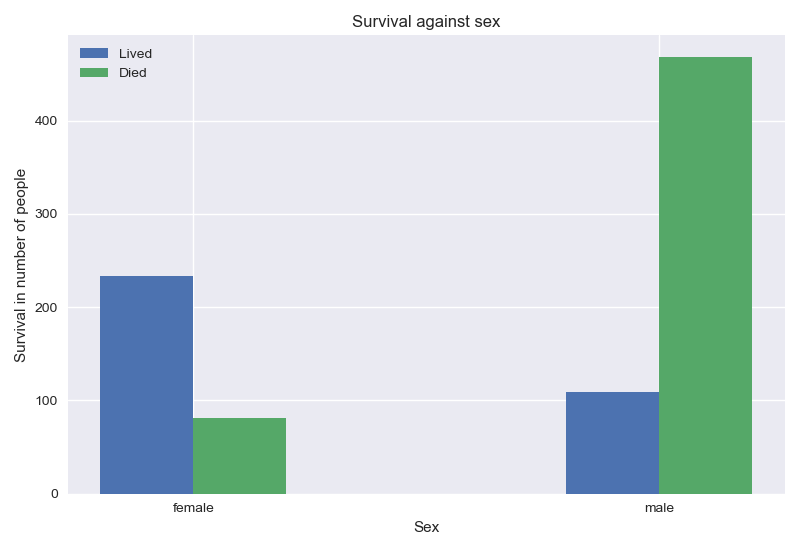
Compared to men, women had a better chance of survival
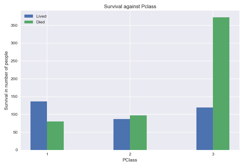
From the graph above, passengers on first and second class had a better chance of survival.
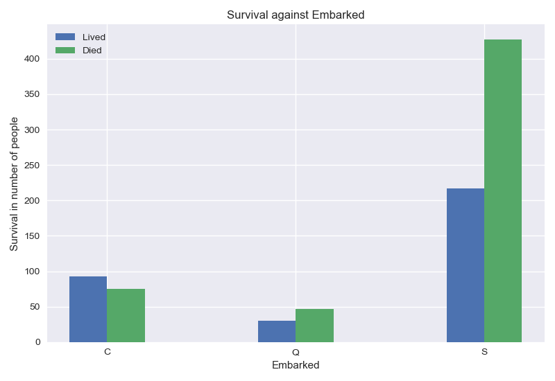
I don’t really know how to interpret the Embarked feature. Does the embarkation port explain survival ? Correlation and causality are quite different. I will keep the feature for now, but I will test with and without it.
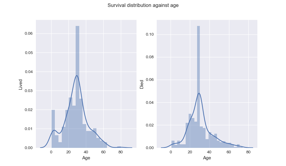
From Age distribution, we can see that indeed, children had better chance of survival.
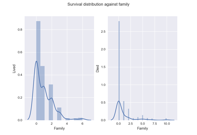
Instead of keeping Parch and SibSp: , I create the new feature Family, to describe number of family members on board.
data["Family"] = data["Parch"] + data["SibSp"]
data.drop(["SibSp", "Parch"], axis=1, inplace=True)
As for Ticket and Cabin, I decide to drop them.
Can the cabin explain the survival rate ? We can imagine that the closer the cabin is to the life boat, the better is the chance of surviving, but as there are 687 empty Cabin values, I doubt there is a good way to fill these missing values.
As for Ticket, I think the Pclass already brings a more general information of that. Plus, it is difficult to manage it.
data.drop(["Ticket", "Cabin"], axis=1, inplace=True)
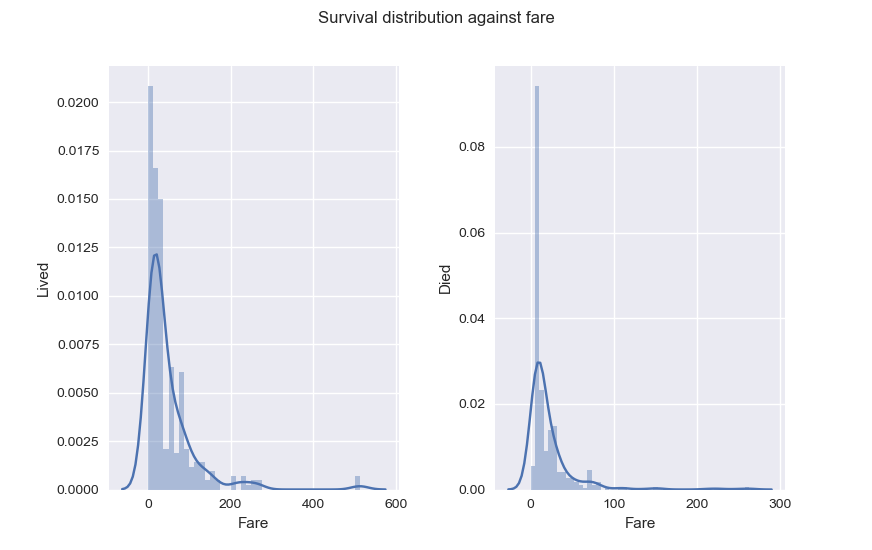
As for Fare, it seems passengers with higher Fare had better chance of Survival. Also, something you should know and that explains why Fare distribution is skewed to the right : Fare for passengers in the same family is a sum of all their tickets fares. That will be very helpful later.
Missing values
To fill missing values, I choose the mean for Age and Fare, most frequent value for Embarked.
# Replace age = nan values with median or mean, median as there are some zeros.
# Replace embarked = nan embarked with most frequent value
# Replace fare = nan with mean
data["Age"] = data["Age"].fillna(data["Age"].mean())
data["Fare"] = data["Fare"].fillna(data["Fare"].mean())
data["Embarked"] = data["Embarked"].fillna(data["Embarked"].value_counts().index[0])
Adding new features
It is clear that I wouldn’t keep Name as feature, however the name has an information worth considering, the title : Mr, Mrs, Col, Don … Not only it gives an idea about the sex but also the marital status and the rank in society at that time.
# Create a new feature = Title
data["Title"] = data.Name.str.split(', ', expand=True)[1].str.split('.', expand=True)[0]
data["Title"].replace("Mlle", "Miss", inplace=True)
data["Title"].replace(["Ms", "Mme"], "Mrs", inplace=True)
data["Title"].replace("Don", "Master", inplace=True)
data["Title"].replace(["Capt", "Col", "Major"], "Military", inplace=True)
data["Title"].replace(["the Countess", "Sir", "Lady","Dona","Jonkheer"], "Elite", inplace=True)
Also, if we regroup passengers of the same family (meaning who have the same last Name and the same Fare), we can see a passenger’s survival is related to his/her relatives survival (credit for the idea).
If all of relatives didn’t survive, he/she has a bigger chance of not surviving.
If at least one of relatives survives, he/she has a bigger chance of surviving.
Below examples with some families from the train data set.
Survived  max      0.0
          count    4.0
          mean     0.0
Name: (Palsson, 21.075)
Survived  max      0.0
          count    6.0
          mean     0.0
Name: (Panula, 39.6875)
Survived  max      0.0
          count    5.0
          mean     0.0
Name: (Rice, 29.125)
Survived  max      1.0
          count    3.0
          mean     1.0
Name: (Richards, 18.75)
Survived  max      0.0
          count    7.0
          mean     0.0
Name: (Sage, 69.55)
Survived  max      0.0
          count    6.0
          mean     0.0
Name: (Skoog, 27.9)
Survived  max      1.000000
          count    3.000000
          mean     0.666667
Name: (Taussig, 79.65)
Survived  max      1.000000
          count    3.000000
          mean     0.666667
Name: (Thayer, 110.8833)
Survived  max      0.0
          count    3.0
          mean     0.0
Name: (Van Impe, 24.15)
Survived  max      0.0
          count    3.0
          mean     0.0
Name: (Vander Planke, 18.0)
Survived  max      1.000000
          count    3.000000
          mean     0.666667
Name: (West, 27.75)
def add_survival_rate(train, test):
    train['LastName'] = train.Name.str.split(', ', expand=True)[0]
    test['LastName'] = test.Name.str.split(', ', expand=True)[0]
    cols = dict(max='max', count='count')
    rate = train[["Survived", 'LastName', 'Fare']].groupby(['LastName', 'Fare']).agg(cols.keys())
    # to initialize in case there is a family in test not in train, or for people with no family in train
    train["Rate"] = 0.5
    test["Rate"] = 0.5
    for index, row in rate.iterrows():
        if row.iloc[1] != 1:
            train.loc[(train.LastName == index[0]) & (train.Fare == index[1]), "Rate"] = row.iloc[0]
            test.loc[(test.LastName == index[0]) & (test.Fare == index[1]), "Rate"] = row.iloc[0]
    # drop name, fare as not needed anymore
    train.drop(["Name","LastName","Fare"], axis=1, inplace=True)
    test.drop(["Name","LastName","Fare"], axis=1, inplace=True)
    return train, test
Transforming features
The goal is to transform categorical features to numeric features using one hot encoding (for binary or ordered features) or dummy features. I test both and the results in accuracy after modeling are similar.
I prefer to transform such variables into binary features, it adds more columns but it is still acceptable in this case.
# Convert to dummy variables.
data = pd.get_dummies(data=data, columns=["Sex", "Embarked","Title"])
If you would like to experiment with the other solution, here is an example for Sex and Embarked features.
# replace string categorical values with int : Sex, Embarked.
data["Sex"].replace("male", 1, inplace=True)
data["Sex"].replace("female", 2, inplace=True)
data["Embarked"].replace("S", 1, inplace=True)
data["Embarked"].replace("C", 2, inplace=True)
data["Embarked"].replace("Q", 3, inplace=True)
Scaling
Since features are on different scales, this step is important. I scale both training and testing sets using the mean and standard deviation of the training set.
def scale(train, test):
 means = train.mean()
 stdevs = train.std()
 train = (train.subtract(means,axis=1)).divide(stdevs,axis=1)
 test = (test.subtract(means,axis=1)).divide(stdevs,axis=1)
 return train, test
Modeling
Let’s start the fun part, which is exploring machine learning algorithms.
Since the training data set is small (891 rows) and there is a limited number of features (6 if OHE or 14 using the dummy transformation), a good classification algorithm to try is support vector machine, SVM with Gaussian kernel.
But first, let’s split the training set into a training set and a cross validation set. The cross validation error would be a great indicator of how the model performs on data it has never “seen”. Also, the comparison between the training error and cross validation error helps to check if there is over fitting.
X_train, X_test, y_train, y_test = model_selection.train_test_split(X_scaled,y,test_size=0.3)
range_C = 2. **np.arange(-3,3,0.1)
range_g = 2. **np.arange(-3,3,0.1)
param_grid = {'C': range_C, 'gamma': range_g}
grid_search = model_selection.GridSearchCV(svm.SVC(kernel='rbf'), param_grid, cv=5, scoring='f1')
grid_search.fit(X, y)
The scoring method is f1_score.
I test the model’s accuracy with and without Embarked, the results are similar. This is a fair proof that a high correlation between a feature and the predicted variable doesn’t mean there is causality and doesn’t give reason to remove/keep features (just because they are/aren’t highly correlated with the explained variable).
F1 score on train set : 0.8032128514056226
F1 score on cv set : 0.8244274809160305
Prediction
y_pred = classifier.predict(X_pred_scaled)
y_pred = pd.DataFrame(y_pred, columns=["Survived"])
y_pred.insert(0, "PassengerId", data_test["PassengerId"])
y_pred.to_csv("pred.csv", index=False)
The accuracy on the test set on Kaggle is 0.81339 (Top 5%).
Thanks for reading this post and see you soon !

hi there, your article is amazing.Following your news.